Single Table Design — AWS DynamoDB

Why, How, What, Where!

Its time to make use of Partitions

Background

NoSQL databases are purpose built for specific data models and have flexible schemas for building modern applications. NoSQL databases are widely recognized for their ease of development, functionality, and performance at scale.

In this article, let’s talk about NoSQL.

• Flexibility: NoSQL databases generally provide flexible schemas that enable faster and more iterative development. The flexible data model makes NoSQL databases ideal for semi-structured and unstructured data.
• Scalability: NoSQL databases are generally designed to scale out by using distributed clusters of hardware instead of scaling up by adding expensive and robust servers. Some cloud providers handle these operations behind-the-scenes as a fully managed service.
• High-performance: NoSQL database are optimised for specific data models and access patterns that enable higher performance than trying to accomplish similar functionality with relational databases.
• Highly functional: NoSQL databases provide highly functional APIs and data types that are purpose built for each of their respective data models.

Types of NoSQL Databases we had to choose from:

• Key value: Amazon DynamoDB.
• Document: Amazon DocumentDB
• In-memory: Amazon Elasticache
• Search: Amazon Elasticsearch Service
• Graph: Amazon Neptune.
• Timeseries: Amazon Timestream.
• Ledger: Amazon Quantum Ledger Database (QLDB)

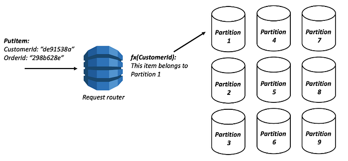
We chose Amazon DynamoDB as they are highly partition-able and allow horizontal scaling at scales that other types of databases cannot achieve. And they are designed to provide consistent single-digit millisecond latency for any scale of workloads.

Another key feature Dynamo Streams give the benefit of capturing changes to items stored in a DynamoDB table, at the point in time when such changes occur using events.

DynamoDB Streams captures a time-ordered sequence of item-level modifications in any DynamoDB table and stores this information in a log for up to 24 hours. Applications can access this log and view the data items as they appeared before and after they were modified, in near-real time

Once we decided on DynamoDB, we could have easily gone down the path of creating a relational structure by creating a table per domain entity but thanks to Rick Houlihan, Inventor of #SingleTableDesign we now have only one table with millions of records of data spread across indexes belonging to various domain entities providing millisecond latencies.

We will help understand how do we achieve this with a single table design for a complex domain model such as ours

Section 1: Why this pattern has been invented?

References:
https://www.alexdebrie.com/posts/dynamodb-single-table/

Reason behind this pattern: To retrieve multiple, heterogeneous item types using a single request.#Fast_retrieval #High_Performance #Think_more while_putting_data

Basic design philosophy in Relational DBs
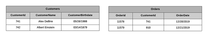
With relational databases, you generally normalize your data by creating a table for each type of entity in your application.

For example:
Customers and one table for Orders.

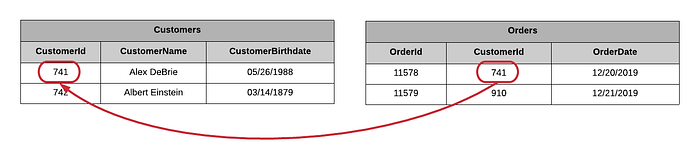
To follow these pointers, the SQL language for querying relational databases has a concept of joins. Joins allow you to combine records from two or more tables at read-time.

Why DynamoDB doesn’t have SQL joins?

SQL joins are also expensive. They require scanning large portions of multiple tables in your relational database, comparing different values, and returning a result set.

DynamoDB was built for enormous, high-velocity use cases, such as the Amazon.com shopping cart. These use cases can’t tolerate the inconsistency and slowing performance of joins as a datasets scales.

DynamoDB closely guards against any operations that won’t scale, and there’s not a great way to make relational joins scale. Rather than working to make joins scale better, DynamoDB sidesteps the problem by removing the ability to use joins at all.

Here comes Single Table Pattern!

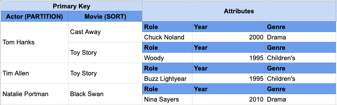
The terminology to define a group of related data within a single table is called as Item collection.

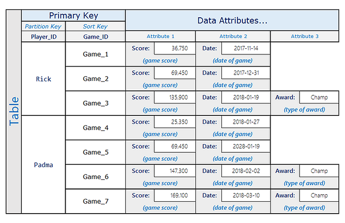
An Item collection in DynamoDB refers to all the items in a table or index that share a partition key. In the example below, we have a DynamoDB table that contains actors and the movies in which they have played. The primary key is a composite primary key where the partition key is the actor’s name and the sort key is the movie name.

Section 2: What are its advantages and disadvantages?

Advantages:

1. Reducing the number of requests for an access pattern is the main reason for using a single-table design with DynamoDB
2. To configure alarms, monitor metrics, etc. If you have one table with all items in it rather than eight separate tables, you reduce the number of alarms and metrics to watch.
3. Having a single table can save you money as compared to having multiple tables.

Disadvantages:

• The steep learning curve to understand single-table design
• Difficulty in adding new access patterns
• The difficulty of exporting your tables for analytics

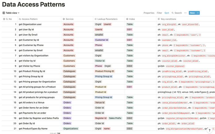
When modeling a single-table design in DynamoDB, you start with your access patterns first. Think hard (and write down!) how you will access your data, then carefully model your table to satisfy those access patterns. When doing this, you will organize your items into collections such that each access pattern can be handled with as few requests as possible — ideally a single request.

NoSQL workbench for DynamoDB is the best tool for data modelling and visualisation.https://docs.aws.amazon.com/amazondynamodb/latest/developerguide/workbench.html

Once you have your table modeled out, then you put it into action and write the code to implement it. And, done properly, this will work great! Your application will be able to scale infinitely with no degradation in performance.

DynamoDB is designed for OLTP (Online Transaction Processing) use cases — high speed, high velocity data access where you’re operating on a few records at a time. But users also have a need for OLAP(Online Analytical Processing) access patterns — big, analytical queries over the entire datasets to find popular items, or number of orders by day, or other insights.

DynamoDB is not good at OLAP queries. This is intentional. DynamoDB focuses on being ultra-performant at OLTP queries and wants you to use other, purpose-built databases for OLAP. To do this, you’ll need to get your data from DynamoDB into another system.

Section 3: Prerequisite knowledge required to understand the implementation

1. Indexing — A data structure technique which allows you to quickly retrieve records from a database file. An Index is a small table having only two columns. The first column comprises a copy of the primary or candidate key of a table. Its second column contains a set of pointers for holding the address of the disk block where that specific key value stored.
2. Inverted Indexing — An inverted index is an index data structure storing a mapping from content, such as words or numbers, to its locations in a document or a set of documents. In simple words, it is a hash-map like data structure that directs you from a word to a document.
3. Primary Index — Primary indexing is defined mainly on the primary key of the data-file, in which the data-file is already ordered based on the primary key.
4. Secondary Index — A secondary index is a way to efficiently access records in a database by means of some piece of information other than the usual primary key.
   As an example of how secondary indexes might be used, consider a database containing a list of students at a college, each of whom has a unique student ID number. A typical database would use the student ID number as the key; however, one might also reasonably want to be able to look up students by last name. To do this, one would construct a secondary index in which the secondary key was this last name.
5. Primary key in Dynamo DB — The primary key can consist of one attribute (partition key) or two attributes (partition key and sort key). You need to provide the attribute names, data types, and the role of each attribute: HASH (for a partition key) and RANGE (for a sort key).
6. Reverse key index — A strategy to reverses the key value before entering it in the index.Ex: the value 24538 becomes 83542 in the index.
   This technique is done to make sure that one particular index data block is not overfilled. Ex: If we have an index on phone number and majority of the number starts from 9 or 8, then there is an overflow in blocks containing numbers starting from 9 and 8.

Section 4: How can we implement this pattern in DynamoDB?

Secondary Indexing in DynamoDB
Amazon DynamoDB provides fast access to items in a table by specifying primary key values. However, many applications might benefit from having one or more secondary (or alternate) keys available, to allow efficient access to data with attributes other than the primary key. To address this, you can create one or more secondary indexes on a table and issue Query or Scan requests against these indexes.

Global secondary index — An index with a partition key and a sort key that can be different from those on the base table. A global secondary index is considered “global” because queries on the index can span all of the data in the base table, across all partitions. A global secondary index is stored in its own partition space away from the base table and scales separately from the base table.

Local secondary index — An index that has the same partition key as the base table, but a different sort key. A local secondary index is “local” in the sense that every partition of a local secondary index is scoped to a base table partition that has the same partition key value.

How can we use the existing Dynamo DB platform to improve our DB performance?

A good document on how we can make use of the Sparse Indexing in Dynamo:
https://docs.aws.amazon.com/amazondynamodb/latest/developerguide/bp-indexes-general-sparse-indexes.html

Improve performance of Aggregation Queries:
https://docs.aws.amazon.com/amazondynamodb/latest/developerguide/bp-gsi-aggregation.html

Section 5: What we do?

Reference:
https://www.serverlesslife.com/DynamoDB_Design_Patterns_for_Single_Table_Design.html

We follow the Single Table pattern in DynamoDB and use Global Secondary Indexes during our CRUD operations.

Principles:

• Put all data in one table or as few as possible.
• Reuse/overload keys and secondary indexes for different purposes.
• Name keys and secondary indexes with uniform names, like PK (partition key), SK (sort key), GS1PK (first global secondary index partition key), GS1SK (first global secondary index sort key).
• Identify the type of the item by prefixing keys with type, like PS: USER#123 (USER = type, 123 = id).
• Duplicate and separate values for keys, indexes from actual application attributes. That means that you can have the same values in two, four, or even more places.
• Add a special attribute to define the type, so the data is more readable.
• Use the partition key that is actually used in access patterns.

Denormalisation

One-to-many relationships are at the core of nearly all applications.

Traditionally to store 1-N relationships in relational world, we would use primary key & foreign key to store related entities for primary record in another table.

In DynamoDB, you have a few different options for representing one-to-many relationships.

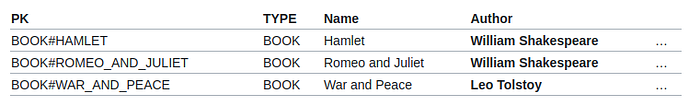
Denormalisation by using a complex attribute

In DynamoDB, we denormalise the data to store in one row by using a complex attribute such as map/list given we don’t have access patterns to get variants by option name for instance in the above screenshot.

Denormalisation by duplicating data pattern

This data is related to other items, so it needs to be duplicated.
If the data is immutable (does not change), there is no problem. But if the data can change, you have to take care of consistency by updating each related record when data changes. We solve this using workers which get triggered on record update via dynamo streams.

Relationship Patterns

Most patterns for modelling a relationship take advantage of the following principals:

• Collocate related data by having the same partition key and different sort key to separate it.
• Sort key allows searching so you can limit which related data you want to read and how much of them (e.g., first 10 records)
• Swap partition and sort key in GSI so you can query the opposite direction of the relationship.

One to Many Relationship Pattern

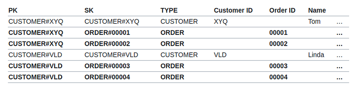
This allows you to:

• Read customer by ID(PK = CUSTOMER#XYQ, SK = CUSTOMER#XYQ)
• Read customer and last 10 orders together(PK = CUSTOMER#XYQ, begins_with("ORDER"),Limit = 11)
• Read only orders of the customer (PK = CUSTOMER#XYQ, SK = begins_with("ORDER"))
• Read order by customer (PK = CUSTOMER#XYQ, SK = ORDER#00001)

Extending the above model using GS1PK and GS1SK (Global Secondary Index)

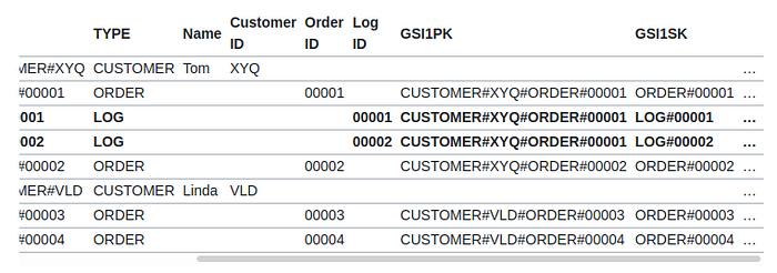
Let’s view the same data from the perspective of GSI:

Conclusion:

We migrated to Single Table architecture 6 months ago from multi table architecture. Our experience have been great so far in terms of performance and code maintenance. A new developer may take some time to find his/her around it but such challenges is what’s helping us grow.